How AFL Supercoach Pricing Works (Part 1)
A data-driven approach to understanding the features of the AFL Supercoach pricing mechanism
--

The AFL Supercoach pricing mechanism is a much simpler implementation of the one used for AFL Fantasy. By comparison, there is also much more written up on the methodology. Hence, this article has been written for the purposes of completeness to my body of work on AFL statistics.
In the same vein as a previous paper on the AFL Fantasy pricing mechanism, this article describes the approach used to backsolve for the formula using inference and statistical techniques — that is, if you didn’t know the formula, how would you go about finding it?
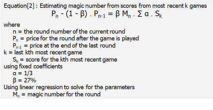
The final model accurately predicts player prices to within 0.05% of the actual next round price using data from more than 85,000 games over the 2010–2019 seasons. The equation and parameters for the pricing model is as follows :

There are many practical applications for using the pricing model, particularly in relation to predicting the path of prices and breakevens through the season which will be a topic to investigate in future analysis.
Linear Regression Hypothesis
The KFC Supercoach guidelines provided a few clues about the pricing mechanism from week to week.
Once a player has played two games their price will change after every game they play after that. A score only stays in a player’s price cycle for three weeks.
The hypothesis for the pricing formula is as follows, and used player data scraped from the footywire web pages from 2010–2019 inclusive, totalling over 85,000 data points.

The approach used was to backsolve for coefficients using a series of linear regressions on the data which progressively simplified the problem. Specifically at the beginning of the exercise, the following calculations and parameters were not fully defined -
- number of game (k) scores which contributed to the score
- the weighting scheme used for each of the most recent scores αₖ
- the weighting of the prices used from previous round β
- the calculation for the magic number Mₙ
The regressions were initially run over season level data and then at the round and player level with to increase accuracy as the parameters and order of calculations became more apparent.
Linear Regression #1 : determining the number of games (k) which contribute to the score
In order to determine the appropriate lookback period I first analysed the contribution of the αₖ coefficients to final price of the equation using k=5.
Analysis of Coefficients From the chart below we see that overfitting or when the coefficients turn from positive to negative occurs after L03 or the 3rd last round played, indicating that k=3 is most ideal to fit the data. Despite the issue of overfitting, both models return an r-squared fit of 99.9% indicating that the pricing mechanism is highly linear.

Analysis of Residual Errors by Number of Regressors An analysis of the predictive errors shows that the regression parameters for the model are different - depending on the number of games played used in the calculations.

Linear Regression #2 : adding number of games played as a model input
Based on these observations the model was updated to use the number of games played as an input — that is, for each round, up to 3 regressions would be run to calculate parameters for each group by number of games played (for k=3).
Hence in the case of R02, a maximum of 2 regressions would be run, taking into account the players who had played 1 or 2 games for the season and for R07, a maximum of 3 regressions would be run. The model was re-run at the season-round level to determine the coefficient of the regressors for up to the last 3 games.

- For the case where less than 3 games have been played (ie number of regressors = 1 or 2) the weights attached to the last k scores = 0%, and to the last price = 100% — confirming that the prices do not change until at least 3 games have been played.
- For the case where 3 games have been played, equal weights are assigned to the last score. One observation is that the weight assigned to the previous price converges to 73% across multiple season-rounds, rather than 75% as one might expect.
The results imply the following table of weights used in the Supercoach pricing formula.

Calculating the Magic Number using fixed weightings of αₖ and β
To confirm if the theory of fixed weights made sense I re-ran the regression using the fixed weights calculated previously, and now allowing the model to imply the magic number directly.
To do this calculation more explicitly, I moved the previous price term from the right hand side of the equation to the left hand side of the equation.

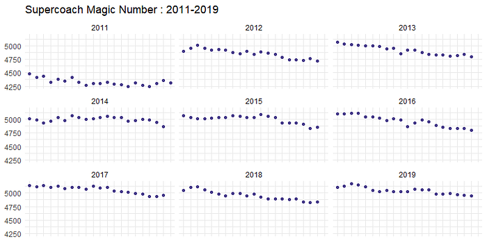
Noting that the magic number is intended to be a rebalancing factor between rounds such that the for a given round, the aggregate of all previous prices is equal to that of all new prices, we can set Pn=Pn-₁ and do all of our calculations based on aggregates for a given round.
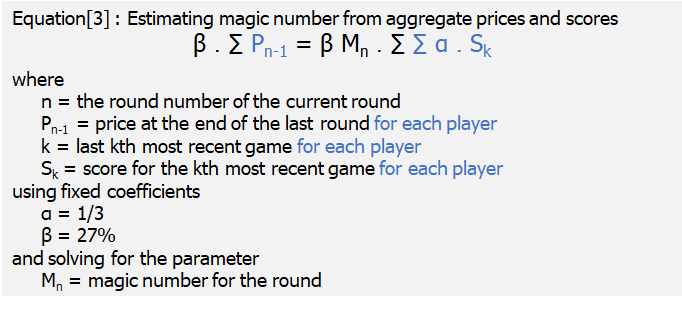
Rewriting equation [2] and aggregating for all players becomes —

In other words, we will calculate the weighted average scores for each player and find the aggregates for that weighted score and the total pre-game prices over the round- which I’ve highlighted in blue to make things clearer.
- This is a very tidy calculation in that we do not have to know the post-game prices in order to find the magic number.
- This formula does not imply that the post-game prices for each player must be equal to their pre-game prices.
- The magic number can only be calculated from R03 onwards when there is a non-zero αₖ value. That is, we have to use the subset of data which comprises only those players who have played at least 3 games. In earlier rounds, we imply the values using a similar calculation philosophy.
No linear regression required here. We only need to backsolve for the magic number given that we know all the other values.

Performance of the Final Model
We now know the values for all of the component parts of the hypothesised model. Putting it all together, we can now assess the quality of model predictions for next price vs actual prices using the original equation [1].
In terms of the actual number of observations by magnitude of absolute errors — out of 85,000 prices predicted over 2010–2019 inclusive, the mean absolute error is less than $300.
Conclusion and thoughts
Linear regression was the statistical technique used to deconstruct the key components of the AFL Supercoach player pricing model. While we used it as a tool to further our understanding of the relationships between prices and scores, the final model does not use any of the actual parameters calculated by the regressions.
There are many practical applications for using the pricing model, particularly in relation to predicting the path of prices and breakevens through the season which will be a topic to investigate in future analysis.
References
- How KFC Supercoach prices work and how to use that to your advantage (link)
